Implement an Analysis
Important
If you have implementations of components, please consider sharing them to help expand and improve COHESIVM. You may also simply propose the implementation of a specific device or interface.
Read the Contributing Guidelines for more information.
This tutorial will guide you through the process of implementing a class for automatized data analysis following
the Analysis abstract base class. To simulate a realistic use case, the tutorials are based
on the measurement of the sheet resistance and resistivity of materials using a four-point probe.
Theory
For the evaluation of the measurement data, we first need to introduce the equations that we will be using. Generally,
two things need to be considered: (i) the relation between the contact distance and film thickness and (ii) the
distance of the contacts from the edge of the sample. Since the film_thickness is only an optional argument in the
FPPMeasurement (see Implement a Measurement), we do not check for the relation of (i) but just implement
both cases (a) thin film and (b) bulk material. For (ii) we consider two additional cases where we introduce imaginary
current source contacts that are mirrored along the sample edge (which is obtained from the
interface_dimensions).
Firstly, we introduce \(l_{mn}\) and \(s_{mn}\) which are distance related factors for the cases (a) and (b), respectively.
These factors are then used in the distance terms for the regular case \(L_0\), \(S_0\) and the edge case
\(L_m\), \(S_m\). The contacts of the current source will be denoted by the indices \(0\) and \(3\),
corresponding to the list indices as defined in the FPP2X2 (see Implement an Interface). Accordingly, the
voltmeter contacts are denoted \(1\) and \(2\), whereas the mirrored current source contacts are \(0_m\)
and \(3_m\).
This leads to the equations for the resistivity \(\rho\) and, if the thickness \(t\) of the film is unknown, the sheet resistance \(R_{\square}\). The measured voltage is denoted by \(V_{12}\) while \(I_{03}\) denotes the measured current.
Analysis Class
The main requirement to follow the Analysis abstract base class are the definition of the
functions and the plots. These dictionaries
tell the parent class and, consequently, the tightly bound AnalysisGUI which methods should be
called for the analysis. For convenience, the result_buffer() can be used to decorate all
methods which follow the functions signature (Callable[[str], DatabaseValue]])
to store already calculated results.
import math
import copy
import numpy as np
import matplotlib.pyplot as plt
from typing import Union, Dict, Tuple, List
from cohesivm.analysis import Analysis, result_buffer
from cohesivm.database import Dataset, Dimensions
from cohesivm.plots import XYPlot
class FPPAnalysis(Analysis):
"""Implements the functions and plots to analyse the data of a four-point-probe measurement
(``FPPMeasurement``).
:param dataset: A tuple of (i) data arrays which are mapped to contact IDs and (ii) the corresponding metadata
of the dataset. Or, optionally, just (i).
:param interface_dimensions: The :class:`~cohesivm.database.Dimensions.Shape` of the interface. Required if the
``dataset`` contains no :class:`~cohesivm.database.Metadata`.
:param contact_position_dict: A dictionary of contact IDs and the corresponding coordinates on the sample.
Required if the ``dataset`` contains no :class:`~cohesivm.database.Metadata`.
:param pixel_dimension_dict: A dictionary of contact IDs and the corresponding
:class:`~cohesivm.database.Dimensions.Generic` shape of the pixels. Required if the ``dataset`` contains no
:class:`~cohesivm.database.Metadata`.
:param temperature: The temperature of the sample during the measurement in K. Required if the ``dataset``
contains no :class:`~cohesivm.database.Metadata`.
:param film_thickness: The thickness of the conductive film in mm. Required if the ``dataset`` contains no
:class:`~cohesivm.database.Metadata`.
"""
def __init__(self, dataset: Union[Dataset, Dict[str, np.ndarray]],
interface_dimensions: Dimensions.Shape = None,
contact_position_dict: Dict[str, Tuple[float, float]] = None,
pixel_dimension_dict: Dict[str, Dimensions.Generic] = None,
temperature: float = None,
film_thickness: float = None,
) -> None:
functions = {
'Temperature (K)': self.temperature,
'Film Thickness (mm)': self.film_thickness,
'Linear Fit Resistance (Ohm)': self.linear,
'Sheet Resistance (Ohm)': self.sheet,
'Film Resistivity (Ohm mm)': self.rho_film,
'Bulk Resistivity (Ohm mm)': self.rho_bulk,
'Edge Distance i0 (mm)': self.edge_dist_i0,
'Edge Distance i3 (mm)': self.edge_dist_i3,
'Edge Sheet Resistance (Ohm)': self.edge_sheet,
'Edge Film Resistivity (Ohm mm)': self.edge_rho_film,
'Edge Bulk Resistivity (Ohm mm)': self.edge_rho_bulk,
}
plots = {
'Measurement': self.measurement,
'Film Resistivity': self.resistance_plot
}
super().__init__(functions, plots, dataset, contact_position_dict)
if self.metadata is not None:
self._interface_dimensions = Dimensions.object_from_string(self.metadata.interface_dimensions)
self._contact_position_dict = self.metadata.contact_position_dict
self._pixel_dimension_dict = {
k: Dimensions.object_from_string(v) for k, v in self.metadata.pixel_dimension_dict.items()}
self._temperature = self.metadata.measurement_settings['temperature']
self._film_thickness = self.metadata.measurement_settings['film_thickness']
else:
self._interface_dimensions = interface_dimensions
self._contact_position_dict = contact_position_dict
self._pixel_dimension_dict = pixel_dimension_dict
self._temperature = temperature
self._film_thickness = film_thickness
self.il = 'Current (A)'
self.vl = 'Voltage (V)'
def temperature(self, contact_id: str = '') -> float:
"""Retrieves the sample temperature from the measurement settings.
:param contact_id: Does nothing.
:returns: The temperature of the sample during the measurement in K.
"""
return self._temperature
def film_thickness(self, contact_id: str = '') -> float:
"""Retrieves the sample film thickness from the measurement settings.
:param contact_id: Does nothing.
:returns: The thickness of the measured conductive film in mm.
"""
return self._film_thickness
@result_buffer
def probe_coordinates(self, contact_id: str) -> List[Tuple[float, float]]:
"""Calculates the absolute coordinates of the four point probe with respect to the interface.
:param contact_id: The ID of the contact from the :class:`~cohesivm.interfaces.Interface`.
:returns: A list of coordinate tuples for the four contacts of the probe.
"""
d = self._pixel_dimension_dict[contact_id]
x_offset, y_offset = self._contact_position_dict[contact_id]
x_abs = [x_offset + x for x in d.x_coords]
y_abs = [y_offset + y for y in d.y_coords]
return list(zip(x_abs, y_abs))
@staticmethod
def line_distance(x1y1: Tuple[float, float], x2y2: Tuple[float, float], xpyp: Tuple[float, float]
) -> Tuple[float, float, float]:
"""Calculates the 2D distance between a line (given by two points) and another point.
:param x1y1: The coordinates of the first point on the line.
:param x2y2: The coordinates of the second point on the line.
:param xpyp: The coordinates of the point for which the distance should be calculated.
:returns: A tuple of the signed distance and the x- and y-component of the normal unit vector.
"""
x1, y1 = x1y1
x2, y2 = x2y2
xp, yp = xpyp
a = y2 - y1
b = - (x2 - x1)
c = -a * x1 - b * y1
m = math.sqrt(a * a + b * b)
a_prim, b_prim, c_prim = a/m, b/m, c/m
dist = a_prim * xp + b_prim * yp + c_prim
return dist, a_prim, b_prim
@result_buffer
def edge_distances(self, contact_id: str) -> Tuple[Tuple[float, float, float], Tuple[float, float, float]]:
"""Calculates the line distances of the closest edge to a four point probe.
:param contact_id: The ID of the contact from the :class:`~cohesivm.interfaces.Interface`.
:returns: A tuple of line distance tuples (see :meth:`line_distance`).
"""
xy = self.probe_coordinates(contact_id)
if_d = self._interface_dimensions
best_dist = (0., 0., 0.), (0., 0., 0.)
# only works with a rectangular interface
if not isinstance(if_d, Dimensions.Rectangle):
return best_dist
edge_vectors = [(0., 0.), (if_d.width, 0.), (if_d.width, if_d.height), (0., if_d.height), (0., 0.)]
min_dist = float('inf')
for x1y1, x2y2 in zip(edge_vectors[:4], edge_vectors[1:]):
dist = self.line_distance(x1y1, x2y2, xy[0]), self.line_distance(x1y1, x2y2, xy[3])
dist_avg = (abs(dist[0][0]) + abs(dist[1][0])) / 2
if dist_avg < min_dist:
min_dist = dist_avg
best_dist = dist
return best_dist
@result_buffer
def mirrored_coordinates(self, contact_id: str) -> List[Tuple[float, float]]:
"""Calculates coordinates for the current source contacts of a four point probe mirrored along the closest
edge.
:param contact_id: The ID of the contact from the :class:`~cohesivm.interfaces.Interface`.
:returns: A list of coordinate tuples for the two mirrored contacts of the probe.
"""
xy_m = self.probe_coordinates(contact_id)[0], self.probe_coordinates(contact_id)[3]
dist = self.edge_distances(contact_id)
return [(xy_m[i][0] - 2 * dist[i][1] * dist[i][0], xy_m[i][1] - 2 * dist[i][2] * dist[i][0])
for i in range(2)]
@staticmethod
def l_mn(xy: List[Tuple[float, float]], m: int, n: int) -> float:
return math.log((xy[m][0] - xy[n][0])**2 + (xy[m][1] - xy[n][1])**2)
@staticmethod
def s_mn(xy: List[Tuple[float, float]], m: int, n: int) -> float:
return math.sqrt((xy[m][0] - xy[n][0])**2 + (xy[m][1] - xy[n][1])**2)
@result_buffer
def l0(self, contact_id: str) -> float:
xy = self.probe_coordinates(contact_id)
return self.l_mn(xy, 1, 0) + self.l_mn(xy, 2, 3) - self.l_mn(xy, 1, 3) - self.l_mn(xy, 2, 0)
@result_buffer
def s0(self, contact_id: str) -> float:
xy = self.probe_coordinates(contact_id)
return -1/self.s_mn(xy, 1, 0) - 1/self.s_mn(xy, 2, 3) + 1/self.s_mn(xy, 1, 3) + 1/self.s_mn(xy, 2, 0)
@result_buffer
def lm(self, contact_id: str) -> float:
xy = self.probe_coordinates(contact_id) + self.mirrored_coordinates(contact_id)
return (self.l0(contact_id)
+ self.l_mn(xy, 1, 4) + self.l_mn(xy, 2, 5) - self.l_mn(xy, 1, 5) - self.l_mn(xy, 2, 4))
@result_buffer
def sm(self, contact_id: str) -> float:
xy = self.probe_coordinates(contact_id) + self.mirrored_coordinates(contact_id)
return (self.s0(contact_id) -
1/self.s_mn(xy, 1, 4) - 1/self.s_mn(xy, 2, 5) + 1/self.s_mn(xy, 1, 5) + 1/self.s_mn(xy, 2, 4))
@result_buffer
def linear(self, contact_id: str) -> float:
"""Performs a linear regression between the measured current and voltage values to obtain the slope, i.e.,
the fitted resistance after Ohm's Law.
:param contact_id: The ID of the contact from the :class:`~cohesivm.interfaces.Interface`.
:returns: The fraction between the measured voltage and sourced current fitted over all data points in Ohm.
"""
return float(np.polyfit(self.data[contact_id][self.il], self.data[contact_id][self.vl], deg=1)[0])
@result_buffer
def sheet(self, contact_id: str) -> float:
"""Calculates the sheet resistance for a probe far from the edge.
:param contact_id: The ID of the contact from the :class:`~cohesivm.interfaces.Interface`.
:returns: The sheet resistance in Ohm.
"""
return abs(4 * math.pi * self.linear(contact_id) * 1 / self.l0(contact_id))
@result_buffer
def rho_film(self, contact_id: str) -> float:
"""Calculates the resistivity of a film for a probe far from the edge.
:param contact_id: The ID of the contact from the :class:`~cohesivm.interfaces.Interface`.
:returns: The film resistivity in Ohm mm.
"""
t = self.film_thickness()
return abs(self.sheet(contact_id) * t) if t is not None else None
@result_buffer
def rho_bulk(self, contact_id: str) -> float:
"""Calculates the resistivity of a bulk material for a probe far from the edge.
:param contact_id: The ID of the contact from the :class:`~cohesivm.interfaces.Interface`.
:returns: The bulk resistivity in Ohm mm.
"""
return abs(2 * math.pi * self.linear(contact_id) * 1 / self.s0(contact_id))
@result_buffer
def edge_dist_i0(self, contact_id: str) -> float:
"""Retrieves the distance of the i0 contact of the four point probe to the closest edge.
:param contact_id: The ID of the contact from the :class:`~cohesivm.interfaces.Interface`.
:returns: The edge distance of the i0 contact in mm.
"""
return self.edge_distances(contact_id)[0][0]
@result_buffer
def edge_dist_i3(self, contact_id: str) -> float:
"""Retrieves the distance of the i3 contact of the four point probe to the closest edge.
:param contact_id: The ID of the contact from the :class:`~cohesivm.interfaces.Interface`.
:returns: The edge distance of the i3 contact in mm.
"""
return self.edge_distances(contact_id)[1][0]
@result_buffer
def edge_sheet(self, contact_id: str) -> float:
"""Calculates the sheet resistance for a probe close to an edge.
:param contact_id: The ID of the contact from the :class:`~cohesivm.interfaces.Interface`.
:returns: The edge sheet resistance in Ohm.
"""
return abs(4 * math.pi * self.linear(contact_id) * 1 / self.lm(contact_id))
@result_buffer
def edge_rho_film(self, contact_id: str) -> float:
"""Calculates the resistivity of a film for a probe close to an edge.
:param contact_id: The ID of the contact from the :class:`~cohesivm.interfaces.Interface`.
:returns: The edge film resistivity in Ohm mm.
"""
t = self.film_thickness()
return abs(self.edge_sheet(contact_id) * t) if t is not None else None
@result_buffer
def edge_rho_bulk(self, contact_id: str) -> float:
"""Calculates the resistivity of a bulk material for a probe close to an edge.
:param contact_id: The ID of the contact from the :class:`~cohesivm.interfaces.Interface`.
:returns: The edge bulk resistivity in Ohm mm.
"""
return abs(2 * math.pi * self.linear(contact_id) * 1 / self.sm(contact_id))
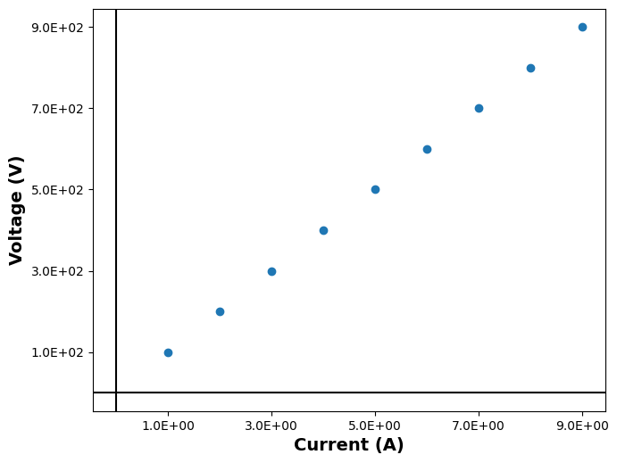
def measurement(self, contact_id: str) -> plt.Figure:
"""Creates a basic x-y plot of the data.
:param contact_id: The ID of the contact from the :class:`~cohesivm.interfaces.Interface`.
:returns: The figure object which may be displayed by the :class:`~cohesivm.gui.AnalysisGUI`.
"""
plot = XYPlot()
plot.make_plot()
data = copy.deepcopy(self.data[contact_id])
plot.update_plot(data)
return plot.figure
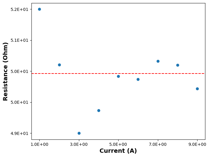
def resistance_plot(self, contact_id: str) -> plt.Figure:
"""Creates a plot of the resistance calculated after Ohm's Law. Should be a horizontal line for the ideal
case.
:param contact_id: The ID of the contact from the :class:`~cohesivm.interfaces.Interface`.
:returns: A figure object which may be displayed by the :class:`~cohesivm.gui.AnalysisGUI`.
"""
plot = XYPlot(origin=False)
plot.make_plot()
data = copy.deepcopy(self.data[contact_id])
data[self.vl] = data[self.vl] / data[self.il]
data.dtype = copy.deepcopy(data.dtype)
data.dtype.names = (self.il, 'Resistance (Ohm)')
plot.update_plot(data)
plot.ax.axhline(y=self.linear(contact_id), color='r', ls='--')
return plot.figure
This is quite a lot, but let’s go through it part by part:
__init__()The constructor of the class takes as required argument the
datasetwhich contains the measurement data together with the correspondingMetadataobject as retrieved byload_dataset(). Optionally, if no metadata is provided, the other arguments must be filled as stated in the docstring. Then, the method defines the availablefunctionsandplotswhich are passed to the parentAnalysis. Finally, measurement and interface properties are stored for later use.
temperature(),film_thickness()These methods are actually just instance properties but they are defined with an optional argument such that they can be used in the
functionsdictionary (which asks for a specific signature).
probe_coordinates(),line_distance(),edge_distances(),mirrored_coordinates()Since the equations above depend on the location of the probe contacts relative to the sample, these methods retrieve and calculate the absolute coordinates of the actual and imaginary/mirrored contacts. The edge with the lowest average distance with respect to the two current source contacts (labels \(0\) and \(3\)) will be selected.
l_mn(),s_mn()The distance related factors \(l_{mn}\) and \(s_{mn}\) are implemented as static methods which take as argument a list of coordinates and the indices for which the factor should be calculated.
l0(),s0(),lm(),sm()These are the distance terms for the four cases which are introduced above: \(L_0\), \(S_0\), \(L_m\), and \(S_m\). They depend on the contact because this defines the absolute coordinates on the interface.
linear()This method is necessary because we measure multiple datapoints and need to extract the fraction \({V_{12}}/{I_{03}}\) which is the slope of the linear fit. It corresponds to the resistance after Ohm’s Law.
sheet(),rho_film(),rho_bulk()These methods extract the resistance/resistivity for the regular case after the equations from above.
edge_dist_i0(),edge_dist_i3()These values help to judge if a probe can be considered close to an edge and support the interpretation of the data.
edge_sheet(),edge_rho_film(),edge_rho_bulk()These methods extract the resistance/resistivity for the edge case after the equations from above.
measurement(),resistance_plot()Finally, the methods for the
plotsare implemented which enable quick inspection of the data (especially in combination with theAnalysisGUI.
Example Usage
Since we implemented the FPPAnalysis to not require a Metadata object, an instance can
be created straightaway. First, we generate some data:
>>> dtype = [('Current (A)', float), ('Voltage (V)', float)]
... d1 = np.array([(a, 100 * a) for a in range(1, 10)], dtype=dtype)
... d2 = d1.copy()
... d3 = np.array([(a, 50 * a + np.random.rand() * 10 - 5) for a in range(1, 10)], dtype=dtype)
>>> dataset = {'P1': d1, 'P2': d2, 'P3': d3}
Then, we define the other arguments and initialize the class:
>>> if_dim = Dimensions.Rectangle(20., 20.)
... con_pos = {'P1': (5., 1.), 'P2': (10., 10.), 'P3': (15., 15.)}
... pix_dim = {k: Dimensions.Generic([-1.5, -0.5, 0.5, 1.5], [0., 0., 0., 0.]) for k in dataset.keys()}
... temp = 300.
... t = 1.
>>> analysis = FPPAnalysis(dataset, if_dim, con_pos, pix_dim, temp, t)
Finally, we can do some analysis:
>>> analysis.temperature(), analysis.functions['Temperature (K)']()
(300.0, 300.0)
>>> analysis.linear('P1'), analysis.linear('P2'), analysis.linear('P3')
(99.99999999999999, 99.99999999999999, 50.26502217652153)
>>> analysis.sheet('P1'), analysis.sheet('P2'), analysis.sheet('P3')
(453.2360141827193, 453.2360141827193, 227.81918304092616)
As you can see, the methods can either be called directly or by accessing them by their name from the
functions. The linear fit seems to be working since we obtain 100 Ω for P1
and P2, whereas P3 is a little different than 50 Ω from the random noise that we added. Accordingly, the
sheet resistance is approximately half as big for P3 than for the other two probes.
>>> analysis.edge_sheet('P1'), analysis.edge_sheet('P2'), analysis.edge_sheet('P3')
(338.47934651602014, 450.8122096478881, 222.87207821984683)
>>> analysis.probe_coordinates('P1'), analysis.mirrored_coordinates('P1')
([(3.5, 1.0), (4.5, 1.0), (5.5, 1.0), (6.5, 1.0)], [(3.5, -1.0), (6.5, -1.0)])
If we consider the distance between the probes and the edge of the sample, clearly, the resistance for P1 is much
smaller but the values for the other two probes barely change. We then confirm that the coordinates of the current
sourcing contacts are correctly mirrored.
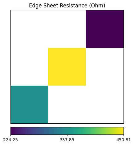
>>> result_map = analysis.generate_result_maps('Edge Sheet Resistance (Ohm)')[0]
... result_map
array([[338.47934652,          nan,          nan],
       [         nan, 450.81220965,          nan],
       [         nan,          nan, 224.91600737]])
The generate_result_maps() returns an array where the values are placed according to
their location on the sample/interface. The resulting array does not capture the exact distances because the contacts
are placed irregularly but it delivers qualitatively the correct positions. We can use the
plot_result_map() to plot it:
from cohesivm.analysis import plot_result_map
plot_result_map(result_map, 'Edge Sheet Resistance (Ohm)')
To conclude, let’s visualize the data using the methods defined in the plots:
>>> analysis.measurement('P1')
... plt.show()
>>> analysis.resistance_plot('P3')
... plt.show()