Analysis GUI
This Graphical User Interface enables to plot measurement data and display analysis results.
Environment
Important
In order to work with the graphical user interfaces, you will need the gui extra. If you installed only the core
package, run the following command to get all required dependencies:
pip install cohesivm[gui]
We use the code from the test of the AnalysisGUI for demonstrating its functionality:
import cohesivm
import numpy as np


class DemoAnalysis(cohesivm.analysis.Analysis):

    def __init__(self, dataset, contact_positions=None):
        functions = {
            'Maximum': self.max,
            'Minimum': self.min,
            'Sum': self.sum,
            'Dot Product': self.dot_product,
            'Average': self.average
        }
        plots = {
            'Measurement': self.measurement,
            'Semilog': self.semilog
        }
        Analysis.__init__(self, functions, plots, dataset, contact_positions)
        self.x_name = 'a'
        self.y_name = 'b'

    @result_buffer
    def max(self, contact):
        return max(self.data[contact][self.y_name])

    @result_buffer
    def min(self, contact):
        return min(self.data[contact][self.y_name])

    @result_buffer
    def sum(self, contact):
        return sum(self.data[contact][self.y_name])

    @result_buffer
    def dot_product(self, contact):
        return sum(self.data[contact][self.x_name] * self.data[contact][self.y_name])

    @result_buffer
    def average(self, contact):
        return sum(self.data[contact][self.y_name]) / len(self.data[contact])

    def measurement(self, contact_id):
        plot = XYPlot()
        plot.make_plot()
        data = copy.deepcopy(self.data[contact_id])
        plot.update_plot(data)
        return plot.figure

    def semilog(self, contact_id):
        plot = XYPlot()
        plot.make_plot()
        data = copy.deepcopy(self.data[contact_id])
        data[data.dtype.names[1]] = np.log(data[data.dtype.names[1]])
        plot.update_plot(data)
        return plot.figure


x_list = np.linspace(-5, 5, 100)
dtype = [('a', float), ('b', float)]
dataset = {
    '1': np.array([(x, x**2) for x in x_list], dtype=dtype),
    '2': np.array([(x, np.sin(x)) for x in x_list], dtype=dtype),
    '3': np.array([(x, np.cos(x)) for x in x_list], dtype=dtype),
    '4': np.array([(x, np.exp(x)) for x in x_list], dtype=dtype),
    #'5': np.array([(x+10, np.log(x+10)) for x in x_list], dtype=dtype),
    '6': np.array([(x+5, np.sqrt(x+10)) for x in x_list], dtype=dtype)
}

contact_positions = {
    '1': (0., 0.),
    '2': (1., 0.),
    '3': (0., 1.),
    '4': (1., 1.),
    '5': (0., 2.),
    '6': (1., 2.)
}

analysis = DemoAnalysis(dataset, contact_positions)

analysis_gui = cohesivm.gui.AnalysisGUI(analysis)
analysis_gui.display()
In order to work with this GUI, an Analysis must be implemented first, which is covered in
detail in the tutorial Implement an Analysis. Then, we generate the dataset where we set the dtype according
to how it’s defined in the DemoAnalysis. Since we do not implement an Interface and
do not have a Metadata object, we must define contact_positions for initializing
the Analysis.
Usage
When you run this code in a Jupyter Notebook, the following GUI should be displayed:
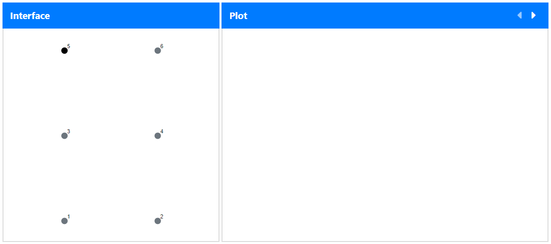
Similar to the ExperimentGUI, we have an Interface and a Plot panel on the left and right
side, respectively. The former one only contains the representation of the contact_positions which we defined above
and the other one is currently empty.
The black dot, labelled ‘5’, indicates that no data entry is available for this contact ID (which is how we defined
the dataset above). If you click on a gray dot, however, it will turn blue and the measurement data will appear in
the plot panel. Additionally, the functions and their results are tabulated in the bottom of the GUI:
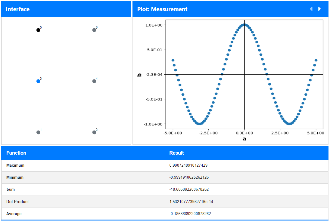
If you look back at the implementation of the DemoAnalysis, you can see that these functions are exactly the ones
we specified in the __init__(). The currently displayed plot corresponds to the measurement() which can be
changed to the semilog() in the Plot panel by clicking the right-arrow in the top right.