Real-World Example
This tutorial provides a high-level description of using COHESIVM, based on a real-world example.
Sample and Measurement Setup
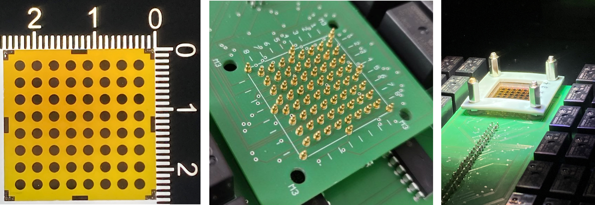
The sample to be measured is a heterojunction of Ga2O3 and Cu2O thin films deposited on an ITO-covered glass substrate with a size of 25 mm x 25 mm. Details for the preparation and properties of these thin films are described in [DWEW24].
Using the contact mask for the MA8X8 interface, for which the hardware description
is available in the repository, gold is sputtered
on top of the heterojunction to obtain 64 devices. The sample is mounted on the contact interface, with the gold
areas facing the pogo pins. For measuring with and without illumination, the whole interface setup is placed in a
lightproof enclosure, under an Ossila Solar Simulator at the
recommended distance of 85 mm.
The Agilent 4156C Precision Semiconductor Parameter Analyzer,
as implemented in the Agilent4156C device class, is employed to measure
the CurrentVoltageCharacteristic of the heterojunction devices.
Running the Experiment
Exactly like in the Basic Usage example, we begin with importing the required modules and
classes. Depending on the application, only the highlighted lines will be different, because this is where we select
the Device, Interface, and
Measurement for a specific Experiment.
from cohesivm import config
from cohesivm.database import Database, Dimensions
from cohesivm.experiment import Experiment
from cohesivm.progressbar import ProgressBar
from cohesivm.devices.agilent import Agilent4156C
from cohesivm.interfaces import MA8X8
from cohesivm.measurements.iv import CurrentVoltageCharacteristic
Next, we create the Database and give it a meaningful name. At a later stage, we can use
the same file to store measurements of similar samples.
db = Database('Ga2O3-Cu2O-Heterojunction.h5')
We begin the configuration of the components with the Measurement, specifically the
CurrentVoltageCharacteristic as mentioned above. The voltage sweep is setup to start
at -2.0 V and end at 2.0 V, with a step size of 0.01 V. For now, the illuminated parameter is set to
False and we keep the solar simulator off, to obtain the dark current-voltage characteristic (dark IV) curves.
measurement = CurrentVoltageCharacteristic(start_voltage=-2.0, end_voltage=2.0, voltage_step=0.02, illuminated=False)
After initializing the Measurement, we can check the requirements regarding the
Device and the Interface:
>>> measurement.required_channels
[(cohesivm.channels.VoltageSMU, cohesivm.channels.SweepVoltageSMU)]
>>> measurement.interface_type
cohesivm.interfaces.HighLow
This means, that we need a Device with a single Channel which
is either a VoltageSMU or a SweepVoltageSMU.
The InterfaceType of the Interface must be
a HighLow.
Consequently, we initialize the SweepVoltageSMUChannel and inject it
into the initializer of the Agilent4156C.
We also initialize the MA8X8 and provide it the
Dimensions of the sputtered gold areas. The connection parameters are filled utilizing
the config, as described in the Configuration section.
smu = Agilent4156C.SweepVoltageSMUChannel()
device = Agilent4156C.Agilent4156C(channels=[smu], **config.get_section('Agilent4156C'))
interface = MA8X8(pixel_dimensions=Dimensions.Circle(radius=0.425), **config.get_section('MA8X8'))
Lastly, we put all the components together in the Experiment, where we also set the name
of the sample and select to measure at all available contact positions:
experiment = Experiment(
    database=db,
    device=device,
    interface=interface,
    measurement=measurement,
    sample_id='Ga2O3-50c_Cu2O-300s',
    selected_contacts=None
)
For keeping track of the progress, we create a Progressbar and, finally, start
the Experiment:
pbar = ProgressBar(experiment)
with pbar.show():
    experiment.quickstart()
The resulting terminal output should look like this:
Contacts:    25%|████████████████                                               | 16/64 [09:23<28:07,  34.97s/it]
Datapoints:  67%|█████████████████████████████████████████                      | 134/201 [00:24<00:11, 5.74it/s]
For the light IV measurements, we turn on the solar simulator and change the respective setting in
the CurrentVoltageCharacteristic, followed by running the complete script again.
measurement = CurrentVoltageCharacteristic(start_voltage=-2.0, end_voltage=2.0, voltage_step=0.01, illuminated=True)
Data Analysis
To work with the measurement results, we firstly load the Database from before and filter
for the specified sample_id. We obtain a list of strings where each item corresponds to a stored
Dataset.
>>> from cohesivm.database import Database
... db = Database('Ga2O3-Cu2O-Heterojunction.h5')
... db.filter_by_sample_id('Ga2O3-50c_Cu2O-300s')
['/CurrentVoltageCharacteristic/3361670997efa438:26464063430fe52f:d11d583e386e4720:c8965a35118ce6fc:ab60964b1ca23b77:8131a44cea4d4bb8/2024-10-10T13:13:09.028445-Ga2O3-50c_Cu2O-300s',
 '/CurrentVoltageCharacteristic/3361670997efa438:26464063430fe52f:a69a946e7a02e547:c8965a35118ce6fc:ab60964b1ca23b77:8131a44cea4d4bb8/2024-10-10T13:59:17.276789-Ga2O3-50c_Cu2O-300s']
From the datetime at the very end of the strings, we can identify the (older) dark IVs and the (newer) light IVs. For
more complicated scenarios, where more results exist for a single sample_id, it is advisable to filter them based
on the settings, using the
filter_by_settings(), e.g.:
>>> db.filter_by_settings('CurrentVoltageCharacteristic', {'illuminated': True})
['/CurrentVoltageCharacteristic/3361670997efa438:26464063430fe52f:a69a946e7a02e547:c8965a35118ce6fc:ab60964b1ca23b77:8131a44cea4d4bb8/2024-10-10T13:59:17.276789-Ga2O3-50c_Cu2O-300s']
We load the Dataset of the light IV measurements and initialize a
CurrentVoltageCharacteristic, which is an Analysis
specifically for our application:
from cohesivm.analysis.iv import CurrentVoltageCharacteristic
dataset = db.filter_by_sample_id('Ga2O3-50c_Cu2O-300s')[1]
light_iv_dataset = db.load_dataset(dataset)
analysis = CurrentVoltageCharacteristic(light_iv_dataset)
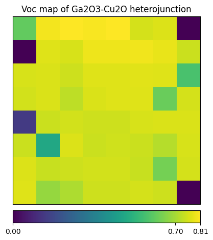
Then, for quickly checking the data, we plot a result map of the open circuit voltage (Voc), using the method referenced
in the functions of the CurrentVoltageCharacteristic:
from cohesivm.analysis import plot_result_map
result_map = analysis.generate_result_maps('Open Circuit Voltage (V)')[0]
plot_result_map(result_map, 'Voc map of Ga2O3-Cu2O heterojunction')
Note
The Analysis is much more powerful in the context of the graphical user interfaces.
Have a look at the description of the Analysis GUI or walk through the Complete GUI Workflow
tutorial to learn more.
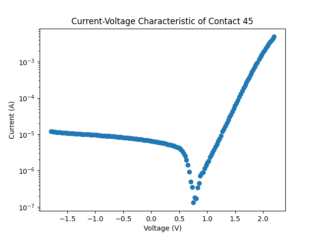
Since the data itself is represented as dictionary of contact IDs that index structured arrays, we select a single measurement curve by its contact ID and plot it using the field names:
import matplotlib.pyplot as plt
contact_id = '45'
measurement_curve = light_iv_dataset[0][contact_id]
x_name, y_name = 'Voltage (V)', 'Current (A)'
plt.scatter(measurement_curve[x_name], abs(measurement_curve[y_name]))
plt.xlabel(x_name)
plt.ylabel(y_name)
plt.yscale('log')
plt.title(f'Current-Voltage Characteristic of Contact {contact_id}')
plt.show()
Closing Remarks
If you want to integrate your laboratory equipment and measurement routines into COHESIVM, learn how to implement your own components in the respective tutorials:
Important
If you have implementations of components, please consider sharing them to help expand and improve COHESIVM. You may also simply propose the implementation of a specific device or interface.
Read the Contributing Guidelines for more information.
Also, have a look on the Complete GUI Workflow to learn how to make use of the graphical user interfaces.
References
Dimopoulos, T., Wibowo, R. A., Edinger, S., Wolf, M., & Fix, T. (2024). Heterojunction Devices Fabricated from Sprayed n-Type Ga2O3, Combined with Sputtered p-Type NiO and Cu2O. Nanomaterials, 14(3), 300. https://doi.org/10.3390/nano14030300